This is a demonstration of the code from the ACM VRST 2008 paper:
Steed, A. (2008) A Simple Method for Estimating the Latency of Interactive, Real-Time Graphics Simulations. ACM Virtual Reality and Software Technology
The code was written for Matlab 7, Release 14. It has not yet been tested with later versions. This code may be used for academic research purposes only. Commercial use requires a commercial licence, please contact the author.
All Downloads
Example videos for sine-fitting (see descriptions below)
Example videos of frame counting (see descriptions below)
Overview of Sine-Fitting Method
The main entry point is the function latency_demo, this takes one or two parameters: the name of a video file and an optional frame offset in to the video file. A typical command would be:
latency_demo(‘cluster_1framea.avi’,100)
where cluster_1framea.avi is the name of a video file (see note below about size and format), and 100 is a number of frame offset in to the video. Thus given one video, you can calculate several estimates of the latency.
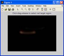
If you run this command, the following window pops up, asking you to select the region containing the red marker. The screen contains a summary of the video of the two pendulums.
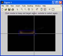
Select the area of the screen containing the red marker – making the region as small as possible, but containing all the red area: this makes the calculation run more quickly. After selecting, you are asked to click in the region to confirm your selection; if you click outside, you can reselect.
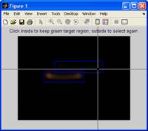
You then do the same for the green region.
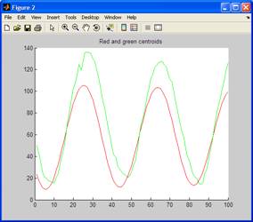
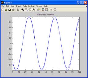
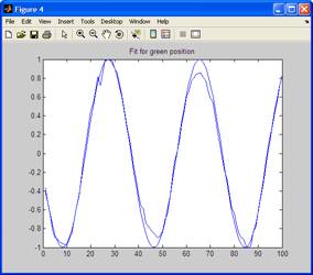
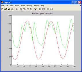
The subsequent calculation can take 20-200 seconds depending on the size of the video regions. It will then show the following three graphs:
Figure 2 is the x position of the extracted centroids of the shape. Figure 3 shows the original x position of the red pendulum and the fitted sine. Figure 4 shows the original x position of the green pendulum and the fitted sine. Here is it important to check that good centroids for the shapes have been found, and that the fits are good.
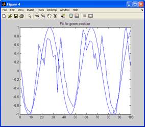
If you don’t select the region accurately you might see in the Figure 2 something like the following:
If the extracted centroids are noisy, then the fit can be bad as shown in the Figure 4 a poor fit. Because there is an optimisation fit of a sine, the fitting can also fail even if the centroids are fine.
In the Matlab window, the output of this particular comand is as follows (some whitespace removed for brevity):
fileName =
cluster_1framea.avi
offSet =
   100
height =
   240
width =
   320
nFrames =
   100
fps =
    25

Optimization terminated: relative function value
 changing by less than OPTIONS.TolFun.
Optimization terminated: relative function value
 changing by less than OPTIONS.TolFun.

frames =
    2.2110
ms =
    0.0884
The last two lines are the latency in number of frames and ms. The calculation is actually done in frames, and relies on the fps marker in the video file to calculate the millisecond offset.
Capturing Videos for Sine-Fitting
There are a few rules of thumb when capturing your own videos. Matlab is not particularly sophisticated in the way it stores and deals with videos. Thus, on my machine, even to get the program to run, I needed to down-size the videos. I did this as explained in the paper. In the download directory, you can find four files:
- cluster_1frame.avi – the original video captured with a web cam
- cluster_1framea.avi – the video downsized to 320×240, de-interlaced
- cluster_5frame.avi – the original video captured with a web cam
- cluster_5framea.avi– the video downsized to 320×240, de-interlaced
you run the Matlab code on the *a.avi files. There are uncompressed video files, this again is a limitation of Matlab – you may have different toolboxes which mean you can use compressed videos. Contact the author if you want more examples of video files.
Advice on setting out the elements in the video is given in the paper.
Code for Sine-Fitting Method
The code is quite simple. If you look at latency_demo.m, you will see the following steps:
  if nargin < 2
      load_video(fileName, 0)
  else
      load_video(fileName, offSet)
  end

  select_regions
  remove_background
  partition_colours
  find_centroids
  smooth_centroids
  fit_sine
if you take videos with different colours, different layouts etc. you will need to change the code. There is an important constraint at the moment, which needs fixing – the red and green regions must not overlap. This is because red and green do not need to be the actual colours red and green, they just need to be bright. The red one is the real pendulum the green the virtual.
Most of the actual computation is dealing with video frames. At the end of smooth_centroids, the progam actually saves enough data to a .mat file, that the subsequent fit_sine method can be recalculated with different parameters. If you are interested in experimenting with this, contact the author, as there are 5 or 6 variations of the fit_sine method using different methods. The one presented is very usable and simple.
The other places that it might be worth taking a look are in the smooth_centroids procedure to remove outliers in blob detection, and the whole blob detection process itself. This just uses standard Matlab functionality, there is certainly more that can be done here.
Examples of Frame-Counting Videos
The frame-counting method is more laborious and uses different videos. These are zip files of .avi files. Unpacked they will be 476MB each. They are mono videos. I have mislaid the sheet with the conversion from name to condition, but here are two examples:


